How search works in Omnesis, and how I made it faster

Omnesis indexes emails, messages, files, calendar events and other personal data so that you or an agent can find things across all of them. But what actually happens between asking a question and getting a list of documents back?

Learning about how to build a search and retrieval system for Omnesis has been incredibly fun and I want to take a bit of time to explain that in this post. I’ll walk through how we prepare documents for search, how full-text search and vector search find different kinds of matches, and how the results come together. I’ll also explain HNSW, the algorithm that makes vector search fast.

Then I’ll finish with a small engineering story of how I was able to optimize full-text search and how it made a large difference in overall search speed on my setup.

There are two ways to find a document

Omnesis combines full-text search, which looks for matching words (a train booking confirmation for example) — where exact match is important, and vector search, which aims to find documents with similar meaning even if none of the words match. I call these “lanes” because each produces its own ranked list of candidates. The pipeline then combines those lists.

For an invented example, searching for “fixing a puncture” might benefit from a document that says “bicycle tyre repair.” A vector match can bridge that difference in wording. But if I remember an exact reference number, I want the full-text lane to find it rather than hope the model considers it similar to something.

Neither kind of match is sufficient on its own. A document can contain my words without answering my question, or be about the right topic without containing the particular fact I need.

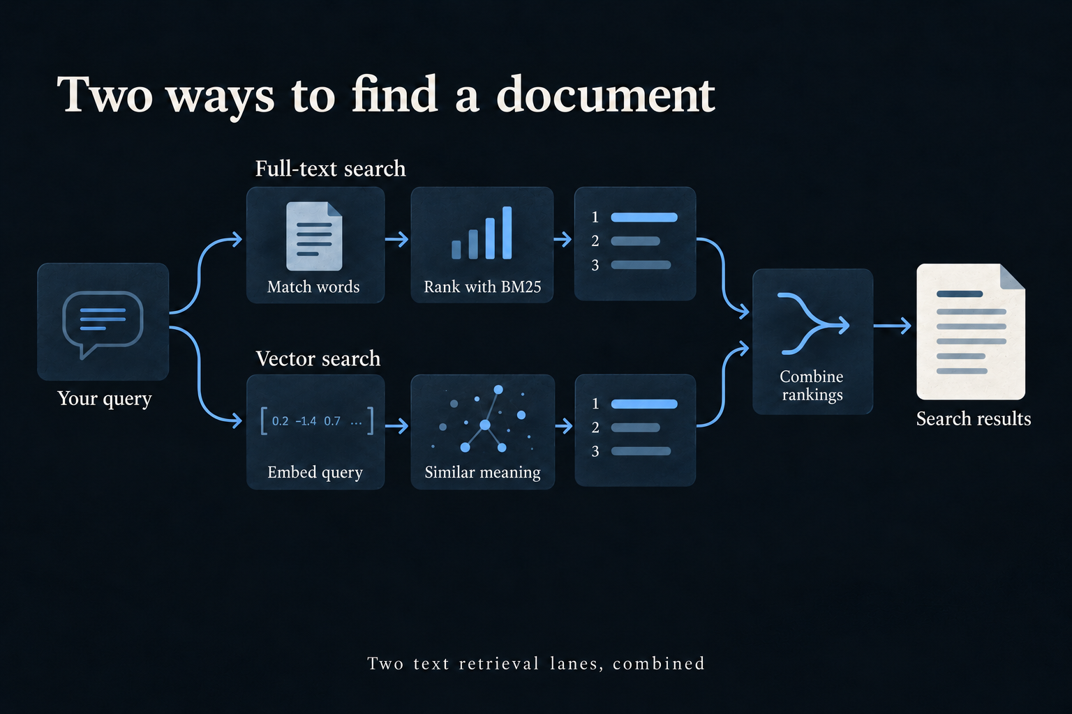
These are the two main text retrieval lanes. Omnesis also has a temporal lane that aims to parse temporal query intents and retrieve select documents from the time index — but I won’t focus on that lane today.

First, do some work before anyone searches

When a document arrives, Omnesis breaks its searchable text into smaller pieces called chunks. A short note might fit in one chunk, while a long document needs several. This lets a relevant passage compete on its own instead of getting lost inside a document about many different things.

The chunks are stored in SQLite with identifiers linking them back to the original document and metadata such as their title and source. From those chunks, the indexer prepares two ways to find them later: a full-text index and a vector index.

The full-text lane

For the full-text lane, Omnesis uses SQLite’s extension called FTS5. FTS5 maps the words into the places where they appear. In search terminology those lists are called posting lists. A search can follow the posting lists for its words instead of opening every chunk and reading it from beginning to end. The extension also tokenizes to normalize the text; for example stemming may let some related word forms match ("running" == "run").

Finding matches is only half the job. If thousands of chunks contain a word, we still need to decide which ones to show first. That is what BM25 does: it assigns a score to each match so that they can be ranked.

The intuition is fairly straightforward. A word that appears in few chunks (such as "Highbury") is usually more informative than one that appears everywhere (such as "the"). Repeating a query word helps, but with diminishing returns: repeating it twenty times should not automatically make a chunk twenty times better. Chunk length matters too, so a long piece of text does not win just because it has more opportunities to contain the word. Omnesis also gives title matches extra weight.

BM25 is arithmetic over word counts and index statistics. Its output is a ranked list of chunk IDs and scores, which can then be connected to the documents those chunks came from.

The vector lane

The vector search lane (also called semantic search) compares numerical representations of text instead of requiring matching words. A model called an embedder converts each chunk and the user’s query into high-dimensional vectors. Think of the numbers in these vectors as coordinates in a space the model has learned: related meanings should be close together, even when the words differ. Omnesis uses cosine distance, which compares their directions: vectors pointing in similar directions are considered close.

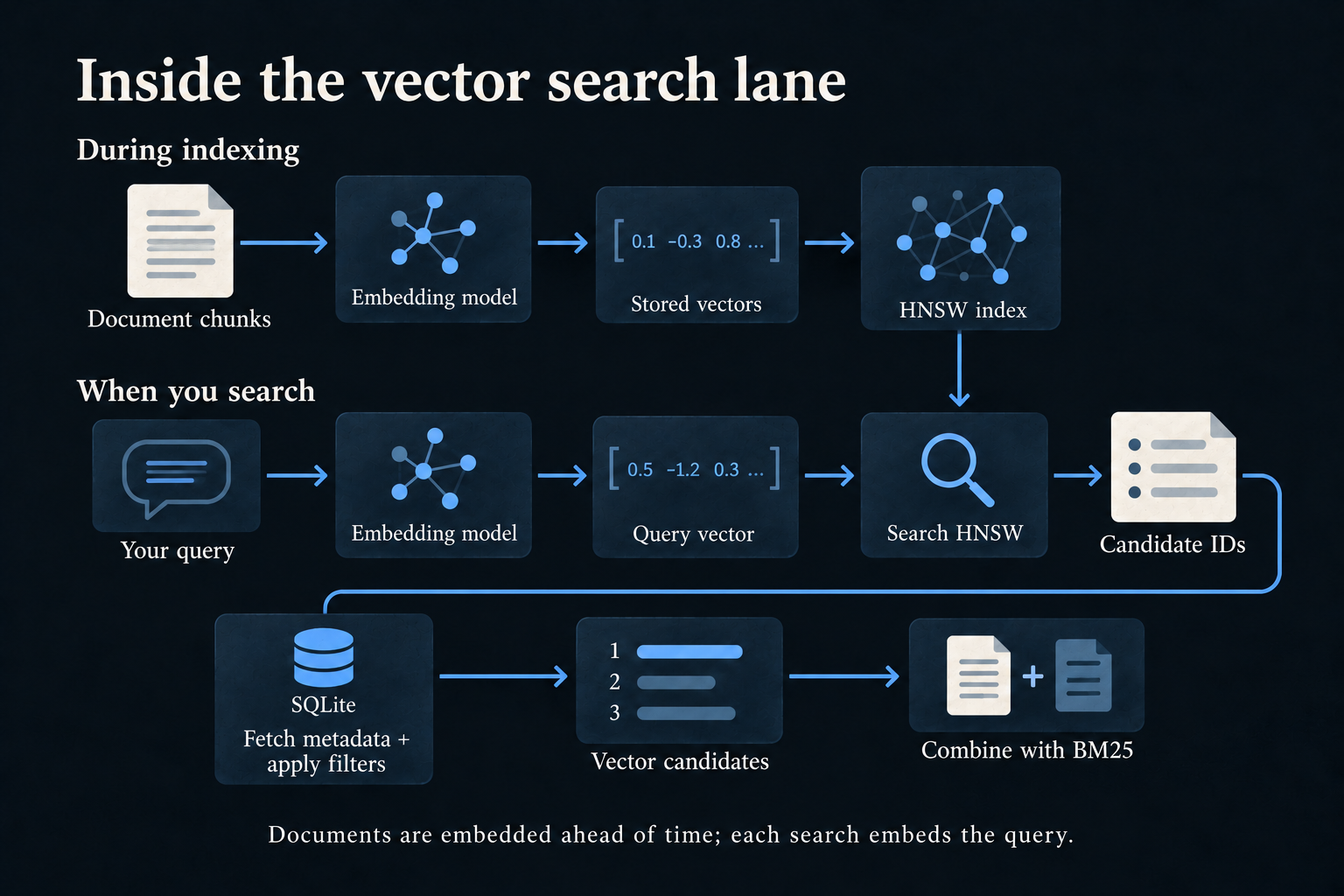
During indexing, Omnesis sends each chunk to the configured embedding model. The input includes a short metadata preamble with context such as the document’s title, type, author and date, followed by the chunk text. That helps preserve some context when a passage is considered separately from its original document.

The resulting embeddings are stored and used to build the vector index. This is work we do when indexing or reindexing documents that changed. Omnesis supports both an in-process embedding model and an HTTP embedding service — allowing the user to run local inference or cloud inference; the vector lane is not tied to one model or one fixed vector size.

At search time, we embed the query. Some retrieval models distinguish between encoding a document and encoding a question, but the results still need to live in a compatible vector space. Changing the embedding model means rebuilding compatible document embeddings, not simply comparing new query vectors with arbitrary old ones.

The simplest vector search would compare the query vector with every stored vector. The work grows linearly with the number of chunks, becoming expensive as the corpus grows. To find neighbours more efficiently, Omnesis uses an algorithm called HNSW via the USearch library.

HNSW: efficiently finding neighbours

HNSW stands for Hierarchical Navigable Small World. Its original paper describes a graph of neighbouring vectors arranged in layers. The base layer contains every indexed vector; the upper layers contain progressively smaller subsets.

Search starts in a sparse upper layer, following links towards vectors closer to the query. It then descends, using the position it reached as the starting point in the next layer. At the base, it explores a set of promising neighbours to produce candidates. Think of the upper layers as shortcuts into a promising neighbourhood, and the base layer as the detailed search within it.

This is approximate nearest-neighbour search: it can miss a true nearest match. Exploring more candidates generally improves recall at the cost of more work. Finding a nearby vector quickly and proving it is the closest vector are different tasks.

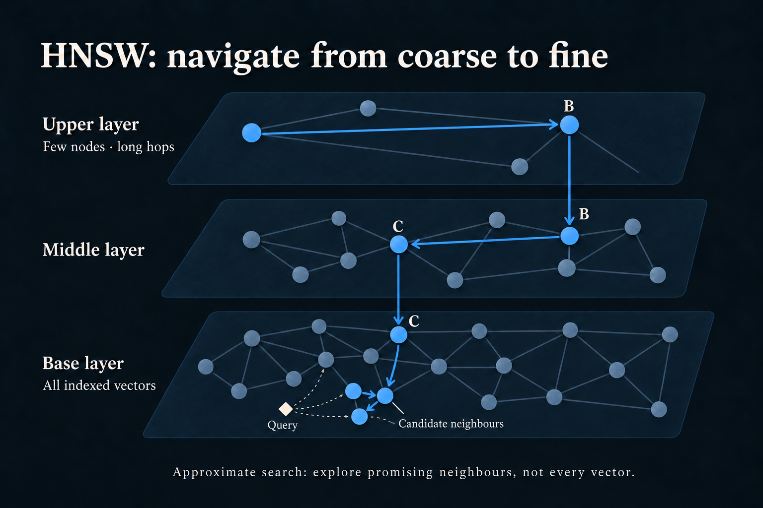
In the diagram, each dot is a chunk vector. The edges help navigate the search index; they are separate from the document and people relationships in Omnesis’s knowledge graph.

In Omnesis, the indexer maintains this graph as vectors are added or removed. Search uses a read view of the saved index. The graph returns chunk identifiers and distances; SQLite supplies the corresponding metadata.

What happens when I add filters?

Search filters let you or an agent restrict results by source, document type, person and other criteria. A nearby vector may belong to a document outside those restrictions.

The vector lane retrieves neighbours first, then fetches their metadata and applies the filters. It asks for extra neighbours to leave room for rejected matches and for multiple chunks from the same document. The pipeline has a default pool of 50 candidates and 10× over-fetch; that means asking for 500 neighbouring chunks. If the explicit filters leave too few candidates, we try once more with a larger request. This work is bounded: we don’t keep widening until we have searched every matching document. A very selective filter can therefore leave the vector lane short of useful results. That is an existing limitation of this approximate retrieval path.

The full-text lane has a different strategy: it can widen its ranked shortlist and fall back to filtering all text matches before choosing the best ones. Person restrictions take that filter-first route directly.

Fusing candidates from the two lanes into search results

We now have two lists, but their raw scores mean different things. A BM25 score describes a word match while a vector score comes from a distance in the embedding space. We cannot directly compare these scores to rank the final search results.

Omnesis combines their rankings using reciprocal rank fusion. Each lane contributes a value based on a candidate’s position in its list, with weights controlling the lanes’ contributions. Ranking near the top contributes more than ranking near the bottom. A chunk found by both lanes receives support from both.

Chunks from the same document are then consolidated so one long document does not occupy the whole results page. Other ranking rules, such as source preferences and optional diversity ordering, can adjust the retained pool. The pipeline fetches text for that pool, removes duplicate content and applies the final result limit.

The small change that made a big difference

Recently I worked on the Omnesis Chrome extension to add the ability to search Omnesis documents directly via Chrome’s address bar, with suggestions as you type. This made the latency of search hard to ignore as some searches took several seconds. It was pretty clear that the culprit was the full-text search lane. I wanted to get search down to something closer to 100–200 milliseconds.

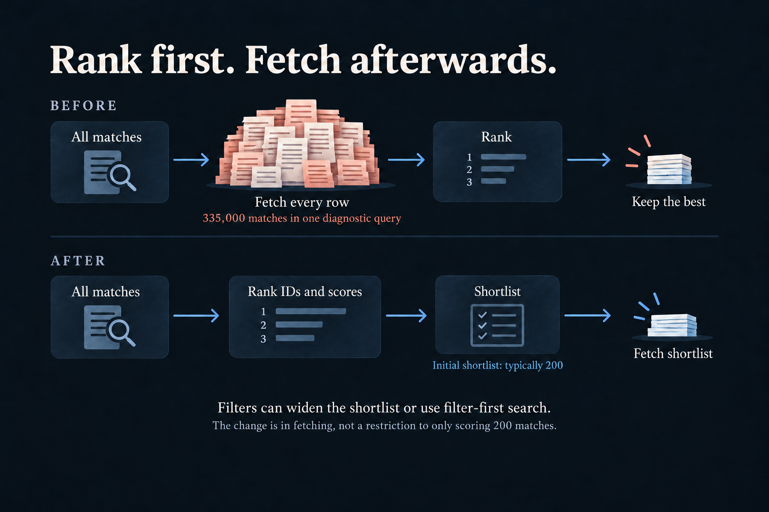
With Claude, we noticed that the SQL query joined every full-text match to the chunks table for metadata and filtering, sorted by BM25 score, and only then kept the winners. It fetched a row for every match before deciding which matches were worth keeping. Asking for a small number of results at the end did not prevent that earlier work.

Even though the query was not selecting the chunk text column, just the metadata lookups meant accessing rows in a large encrypted table. Large rows can occupy multiple database pages, making those lookups more expensive than they look.

In one diagnostic query on my corpus, “the” matched about 335,000 chunks. FTS5 could score them in about 140 ms, but joining each match to its chunk row added roughly 18 microseconds per match. Multiply that tiny cost by 335,000 and you get about six seconds.

Broad queries took 1–8 seconds with a warm cache, and some cold-cache probes took much longer. A warm cache means useful database pages are already in memory; cold runs need more reads from storage. That distinction matters when measuring this change.

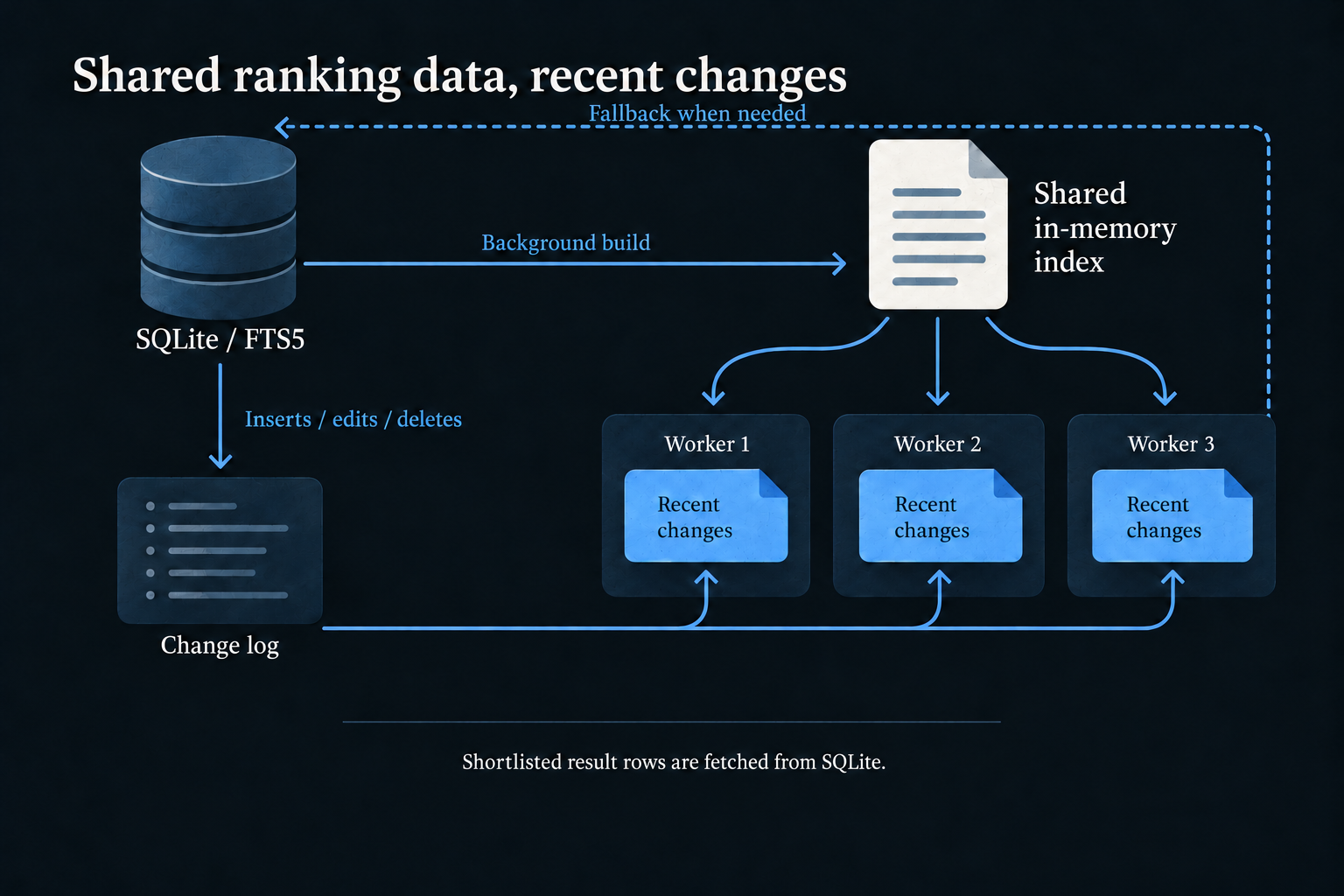
The simple idea was to reverse the order: rank the chunk IDs and scores first, keep a shortlist, then fetch those rows. A typical small search starts with 200 shortlisted chunks. It can still score hundreds of thousands of matches without fetching metadata for every one.

Filters can reject shortlisted results, so the implementation widens the window or falls back to the filter-first query when necessary. The initial 200 are not a hard cutoff that discards every filtered match below them.

We also built an in-memory ranking index from FTS5’s own posting lists. Compact arrays of chunk IDs, word frequencies and length information let the workers compute BM25 without going through SQLite for that step. The search workers share the base index.

This keeps the same scoring formula. On a fixed snapshot, comparing the memory ranker with FTS5 across 1,194 queries gave identical top 50 results, with score differences no larger than floating-point rounding.

On my setup, the copy took about 666 MB and roughly 90 seconds to build in the background. FTS5 serves searches while it builds. Users can disable it with search.bm25.memoryIndex: false and still keep the rank-first improvement.

A database change log lets the rankers follow additions, edits and deletions between rebuilds. If a ranker cannot catch up safely, it falls back to FTS5. The memory index can briefly trail writes, and some statistics refresh only at rebuilds, so fixed-snapshot parity does not promise identical rankings while the corpus changes.

Measuring the impact

The benchmark used my own Omnesis setup and personal corpus. I sampled 380 documents and derived 1,960 queries from them: 1,194 full queries and 766 title prefixes for type-ahead. Those queries ran through the real search pipeline against the corpus; the 380 documents were the sample used to make the queries, not the entire search database.

This is a known-item benchmark: start with a document we know exists, make a query intended to find it, and see what happens. It is useful for measuring whether I can find something I remember having. It is less useful for judging an open-ended question where several different results might be good answers.

Here are the full-search timings reported for the old code and the change that shipped:

Full-search latency	Before	After
Median (p50)	1,306 ms	35 ms
p90	4,173 ms	46 ms
Slowest observed	13,469 ms	159 ms

That is about 37× faster at the median, with the same top 10 results across all 1,194 full queries. Hybrid type-ahead’s median fell from 1,700 ms to 42 ms, making suggestions in my Chrome extension practical!

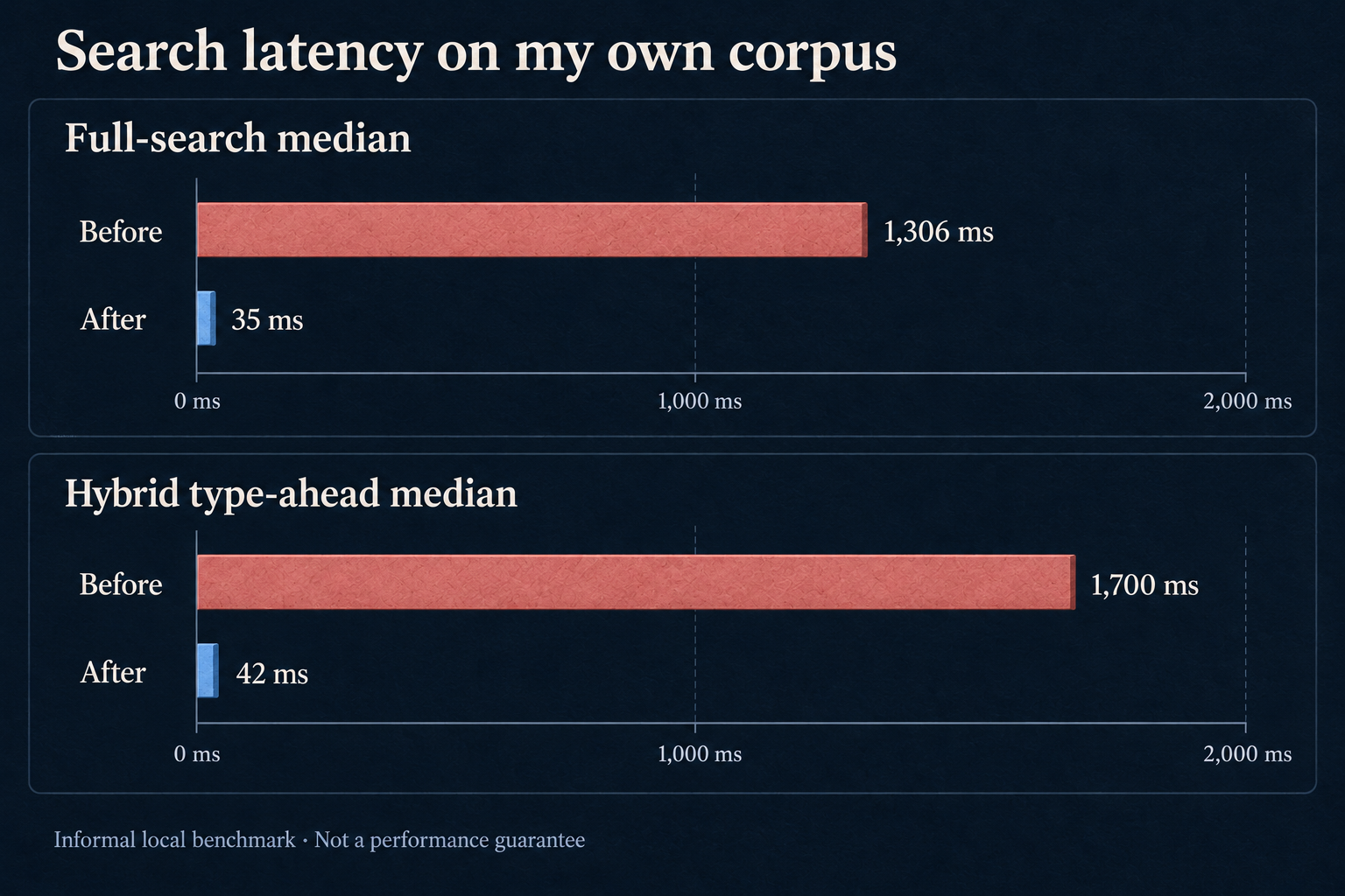
I am very happy with how much faster search feels on my setup. But I want to be open about what these numbers are: this was a vibe benchmark on my own Omnesis corpus, with queries derived from documents already in it. We still need rigorous, representative search-quality evaluations and performance benchmarks.